TABLE OF CONTENTS

Introduction
Quick Overview
Available Models
Acquire NMR data
Process the data in Topspin
Setup the kinetics fitting
Fit the data

Introduction

We have data fitting routines available on the NMRs for your kinetic runs. The programs are written in C++ for integrating the peaks and for fitting the ordinary differential equations of the defined reaction mechanisms. There are several example models available and more can be added as needed for your particular reaction. The integration of the ordinary differential equations is done with the popular 4th order Runge-Kutta method included in ODEINT. Minimization of the target function is done with DLIB using find_min_box_constrained(). You could also try the data fitting with programs such as matlab, R and excel.

Software used:

1. CentOS 7 - The Linux OS which is free
2. Topspin3.6.5 - Bruker NMR software
3. C++ - The programming language
4. Boost - ODEINT comes within Boost for integration.
5. BLAS - Basic Linear Algebra Subprograms.
6. DLIB - is a header only library with many fitting algorithms.
7. Xmgrace - A graphical plot viewer.

*The above programs should all work in the Linux and MacOS environments.

The first part of our tutorial is directed towards people with access to our PC at UIC. Outside users can find the files at the bottom of this page however which includes the Source Code so you can build any model you like and compile. Please note I am very much a novice programmer and any improvements to the code from others would be greatly appreciated. Appendix

A Quick Overview

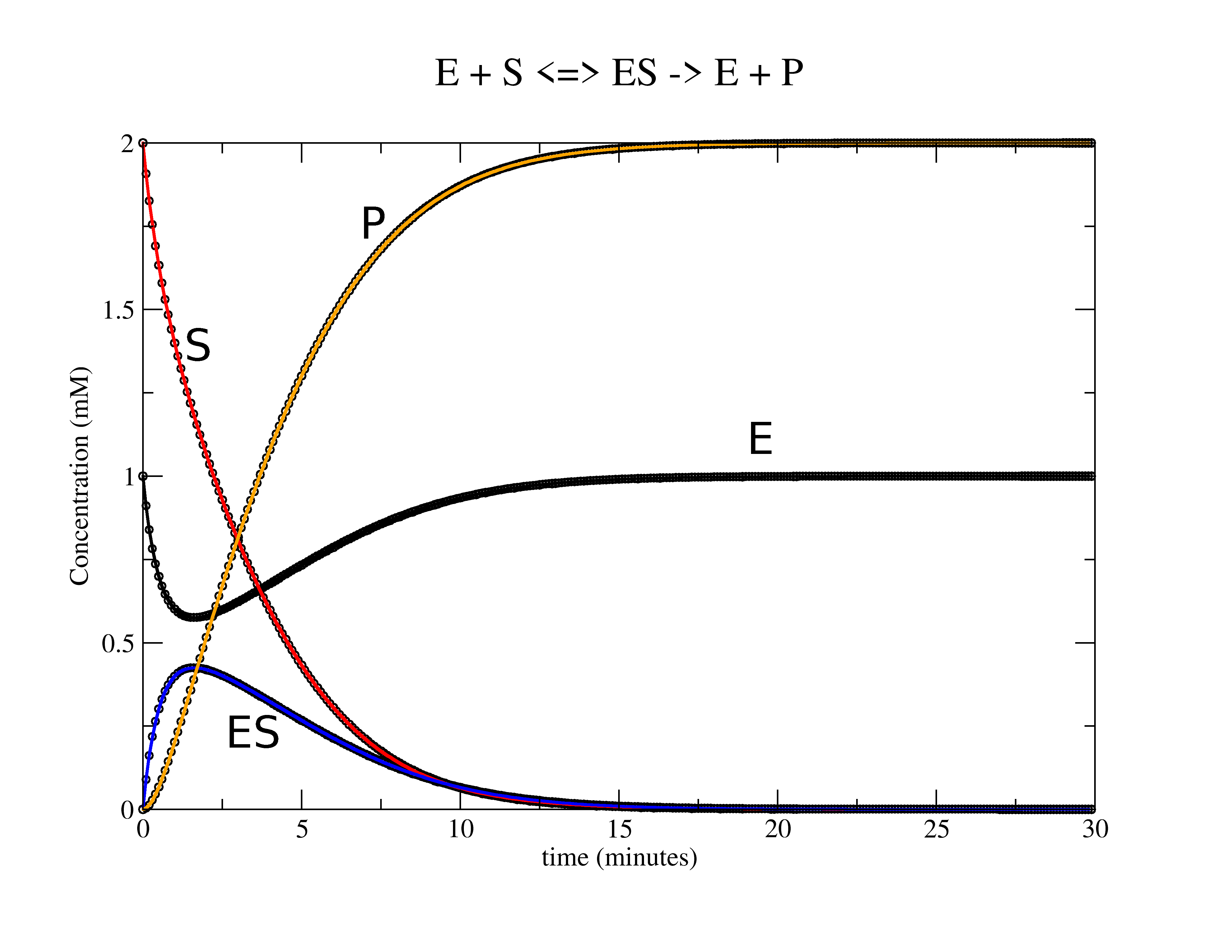
Lets take the standard Michaelis-Menten rxn as an example:

\(\ce{E + S <=>[\text{k1}][\text{k1r}] ES ->[\text{k2}] E + P }\)

or as according to the "dat.txt" columns order

\(\ce{1 + 2 <=>[\text{k1}][\text{k1r}] 3 ->[\text{k2}] 1 + 4 }\)

To use the fitting routine we need 2 files named exactly as below.

• dat.txt -- This is the data block where the first column is "time" and the rest are "intensities". The order matters regarding the columns/peaks.
• guess.txt -- This contains the initial guesses to the rate constants. Hopefully they are close so the program converges better.

Then in a shell/terminal run the program named "kin_sim" :

$ ./kin_sim

 Reading "dat.txt" file. 

 Reading "guess.txt" file for initial rate constants. 

 Saving "results.txt" file with optimal rate constants. 

 Saving "sim.txt" file for simulation curves. 

 k1  = 0.500
 k1r = 0.050
 k2  = 0.750

and the resulting files:

• sim.txt -- The simulated fits to the raw data.
• results.txt -- The 3 rate constants in this example are saved into a results file.

A plot of the resulting data and fits is the top figure above. Note the "initial states" or peak intensities at time = 0 are obtained from the raw data automatically.

Next I'll show how to obtain the "dat.txt" using in-house processing on the NMR directly. However, other methods such as MNova etc are fine to use so long as the data is stored in this block format with the correct column ordering and times.

Models/Mechanisms available so far:

Model1_fit:

\(\ce{A ->[\text{k1}] B}\)

Model2_fit:

\(\ce{A <=>[\text{k1}][\text{k1r}] B}\)

Model3_fit:

\(\ce{A + B <=>[\text{k1}][\text{k1r}] C}\)

Model4_fit:

\(\ce{A + B <=>[\text{k1}][\text{k1r}] C->[\text{k2}]D}\)

Model5_fit:

\(\ce{A + B <=>[\text{k1}][\text{k1r}] C->[\text{k2}]D + A}\)

Acquire Data

After acquiring a simple 1D 1H setup the kinetics run by typing in the Topspin command line kinetic_2d

• AU: kinetic_2d -- answer the questions regarding the delay between expts and number of scans as they pop-up. Type rga and zg afterwards to start the run. pulprog

Topspin Processing

After acquiring the Kinetics data process with:

• xf2 -- Fourier transform in 2nd dimension only
• manually phase the peaks; I leave it to the reader..
• abs2 -- Baseline correction in F2 only
• 2dtxt -- convert the spectra into a text file called "2d.txt". Be sure to define the number of 1Ds you have acquired when prompted.

The "2d.txt" file is saved in the pdata directory in the experiments file name. eg) my folder name is "kinetics_test" and using a shell I find it in:

$ pwd
/home/username/data/dan/kinetics_test/1/pdata
$ ls
1  10  11  12  13  14  15  16  17  2  2d.txt  3  4  5  6  7  8  9  

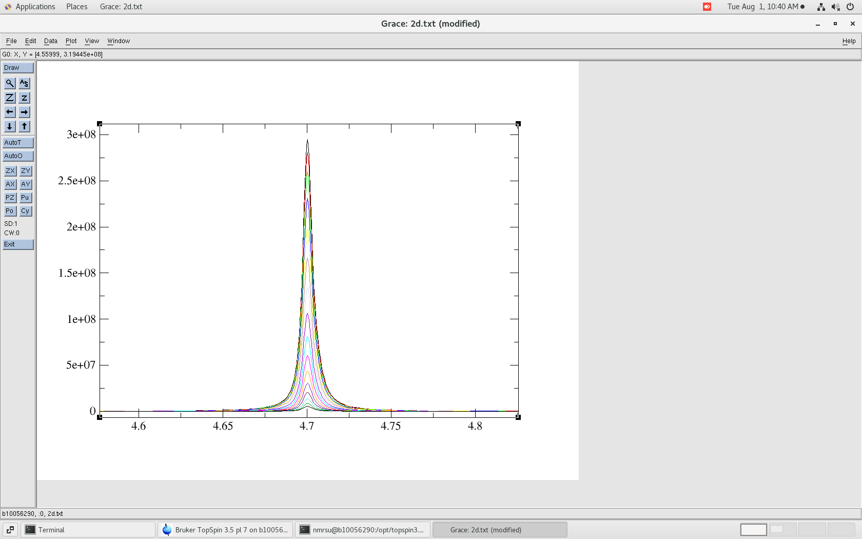
To view lets use the "xmgrace" software:

$ xmgrace ./2d.txt 

The resulting 2d.txt file looks like:

• 2d.txt - The ASCII/TEXT file where the 1Ds are separated by "&"

Copy over your Models fitting directory

Lets copy over the kinetic processing directories into the pdata as well. On our NMRs at UIC I leave some in /opt/processing/kinetics/ eg):

$ ls /opt/processing/kinetics
kinetics_integral  model10      model1_fit  model2_fit  model3_fit  model4_fit  model5_fit
model1             model10_fit  model2      model3      model4      model5      old

And starting from our working processing directory:

$ pwd
/home/nmrsu/data/dan/kinetics_test/1/pdata
$ ls
1  10  11  12  13  14  15  16  17  2  2d.txt  3  4  5  6  7  8  9
$ cp -r /opt/processing/kinetics/model5_fit .
$ ls
1  10  11  12  13  14  15  16  17  2  2d.txt  3  4  5  6  7  8  9 model5_fit 

The "model5_fit" directory is for processing and fitting the kinetics data. The "model5" directory is for performing simulations of the same model via input of the rate constant explicitly. More on this later..

$ cd model5_fit 
$ ls
README  go_int  go_xmgr  guess.txt  kin_sim  mkInteg_kin_cpp  peak.list  scale.txt  src

• README - README file
• go_int - Run the integration routine and generate "dat.txt" file
• go_xmgr - View the resulting fits and data
• guess.txt - Guess the initial rate constants k1/k1r/k2 (is read automatically)
• kin_sim - This is the fitting routine binary file
• mkIntegral_kin_cpp - This is the integrating routine binary file
• peak.list - The peak integral range file
• scale.txt - The peak integral scaling (is read automatically)

Define peaks to fit

We will manually input the peak list ranges that will be integrated and later fitted to a function. eg)

$ gedit peak.list

and when done it looks like:

$ more ./peak.list
0       1.37:1.40
1       2.50:2.53
2       3.62:3.69
3       5.812:6.829

We've defined 4 integral ranges.
The 1st column is the "peak number" corresponding to the first reactant (start at 0)
The 2nd column is the "peak integral range" separated by a ":"

Scale the peaks

This file contains 3 rows for input. Row 2 allows for calibrating an internal control at known concentration. Row 3 is the time step between experiments.

row 1: the number of protons for each peak in list (eg 3 for a CH3)
row 2: first input is known intensity for control(can get from integral), 2nd is the concentration of control (0.1mM here)
row 3: time step between 1Ds (2.0 minutes for example)

$ more ./scale.txt
 1 3 2 2
 7588783298 0.1
 2.0

Note you can just put in all ones to effectively not use this option eg)

$ more ./scale.txt
  1 1 1 1
  1 1
  1.0

And to run the integration routine:

$ ./mkInteg_kin_cpp peak.list ../2d.txt

Reading "scale.txt" file. 

Saving "dat.txt" file used in kinetics simulations 

Resulting in the input "dat.txt" file now calibrated to concentration from the control and known peaks and corrected for the time step between 1D 1Hs.

• dat.txt -- calibrated and ordered for the kinetic simulation data

Fit the data

We have everything now and can start the simulation "kin_sim" :

$ ./kin_sim

 Reading "dat.txt" file.

 Reading "guess.txt" file for initial rate constants.

 Saving "results.txt" file with optimal rate constants.

 Saving "sim.txt" file for simulation curves.

 k1  = 0.500
 k1r = 0.050
 k2  = 0.750

and the resulting files:

• sim.txt -- The simulated fits to the raw data.
• results.txt -- The 3 rate constants in this example are saved into a results file.

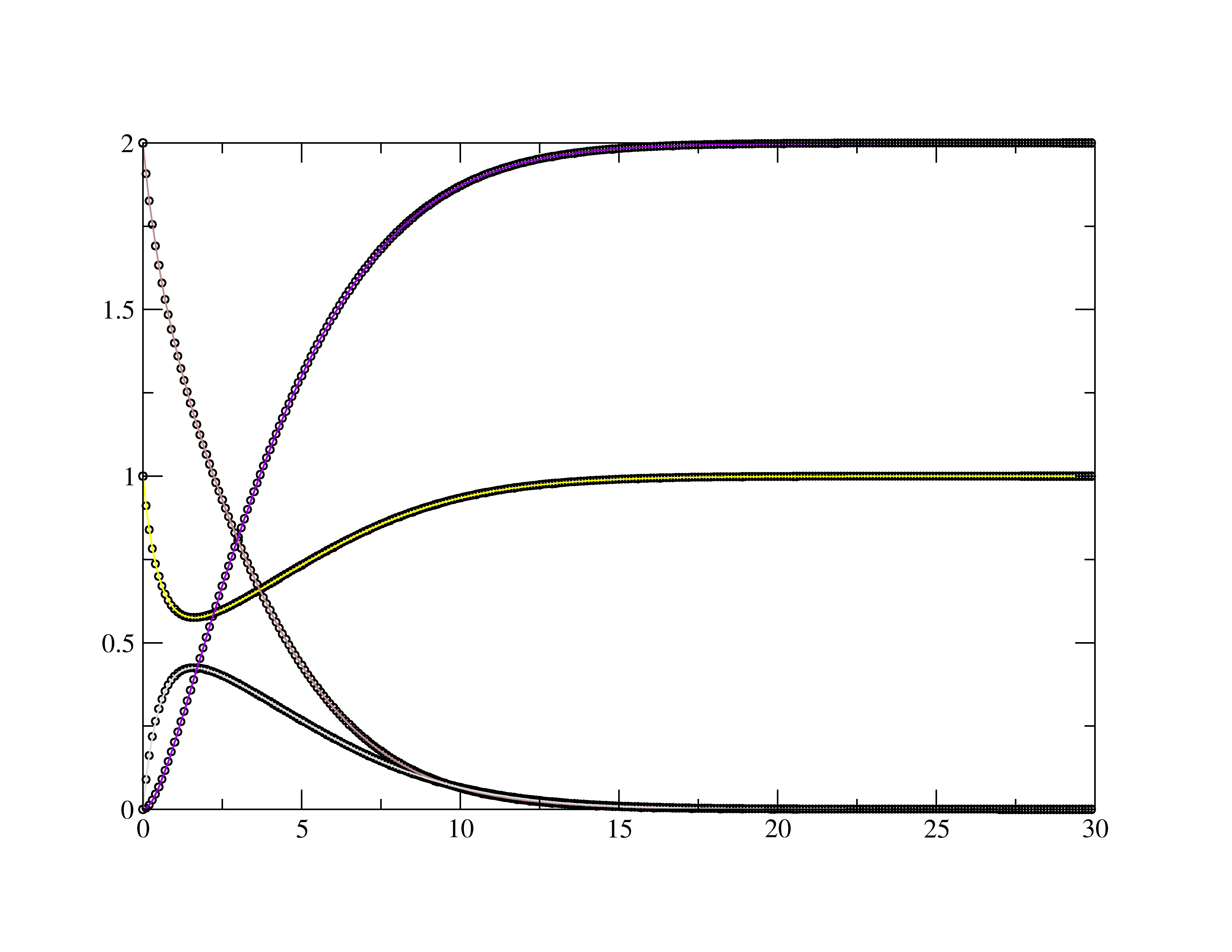
To view output try go_xmgr :

• go_xmgr - View the resulting fits and data

$ ./go_xmgr

Appendix Files:

All of the files and source code for the tutorial are available here: