Introduction

NMR peaks are often overlapped and need to be deconvoluted to extract populations of each component or to resolve the individual contributions of each component to a relaxation rate such as in a T1 study. On our NMRs we can convert the spectra to text files and then run a deconvolution routine written in C++. The peaks are fitted to a Lorentzian model (below) and the minimization of the target function is done with DLIB using find_min_box_constrained().

Software used:

CentOS 7 - The Linux OS which is free
Topspin3.6.5 - Bruker NMR software
C++ - The programming language DLIB - is a header only library with many fitting algorithms.
Xmgrace - A graphical plot viewer.

*The above programs should all work in the Linux and MacOS environments.

The goal now is to recast the spectra into text files and define the peaks to fit. Please note the Source Code is located here so you can build any model you like and compile. Appendix

A Quick Overview

The Absorptive Lineshape being fit for each peak: \begin{equation} {A(\omega)} = {S_0*T_2\over\ 1+(\omega-\Delta\omega)^2*T_2^2} \end{equation}
Lets rewrite it so the fitted variables are hwhh ($LW$) and amplitude $S_0$:

\begin{equation} {A(\omega)} = {S_0*(1/LW)\over\ 1+(\omega-\Delta\omega)^2*(1/LW)^2} \end{equation} and having the parameters:

${\omega}~~~~~~~= \text{current ppm or frequency value}$
${A(\omega)}~= \text{ amplitude at current ppm/frequency}$
${S_0}~~~~~= \text{ maximum amplitude }$
${\Delta\omega}~~~= \text{ frequency offset from on resonance (ppm) }$
${T_2}~~~~~= \text{ $T_2$ time of resonance }$
${LW}~~={1/T2}$

$\text{note: $1/T_2$ = half width half height of peak }$

NMR_class -- for more info on the lineshapes etc please see Chapter_2 notes.

Topspin Processing

After acquiring the Pseudo 2D data process with:

xf2 -- Fourier transform in 2nd dimension only
manually phase the peaks; I leave it to the reader..
abs2 -- Baseline correction in F2 only
2dtxt -- AU to convert the spectra into a text file called "2d.txt". Be sure to define the number of 1Ds you have acquired when prompted.
txt -- AU for 1D data use this command. It saves "2d.txt" file with "&" appended to the end.

The "2d.txt" file is saved in the pdata directory in the experiments file name. eg) my folder name is "kinetics_test" and using a shell I find it in:

$ pwd
/home/username/data/dan/kinetics_test/1/pdata
$ ls
1  10  11  12  13  14  15  16  17  2  2d.txt  3  4  5  6  7  8  9

To view lets use the "xmgrace" software:

$ xmgrace ./2d.txt

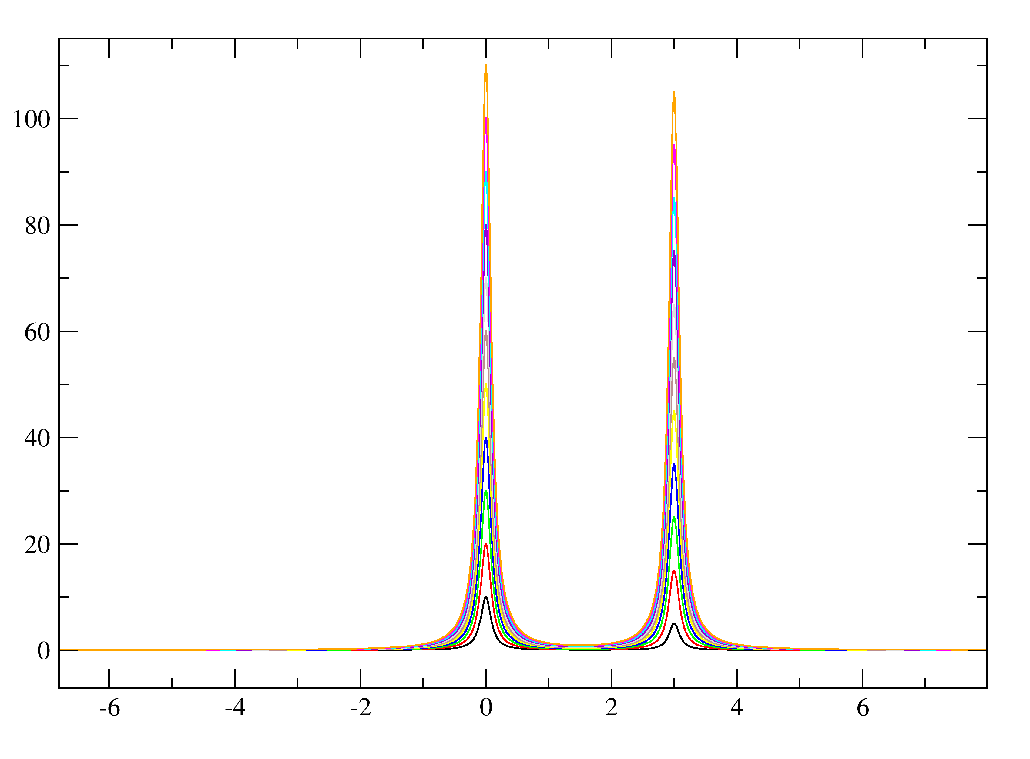
The resulting 2d.txt file looks like:

2d.txt - The ASCII/TEXT file where the 1Ds are separated by "&"

Define peaks to fit

where are we using "pwd" command in shell:

$ pwd
/home/username/data/dan/kinetics_test/1/pdata
$ ls
1  10  11  12  13  14  15  16  17  2  2d.txt  3  4  5  6  7  8  9

The 2d.txt file is now in our "pdata" directory. Lets define the 2 peaks to fit and a range (in ppm) to cut the X-axis.

$ gedit peaks.txt

and when done it looks like:

$ more ./peaks.txt
0.0 3.0
-2. 5.

We've defined:
The 1st row is the peaks to fit in ppm (here 0.0 and 3.0 ppm)
The 2nd row is the cut X-axis range (-2 to 5 ppm)

Deconvolute

We have everything now which is just 2 files "peaks.txt" and "2d.txt".
To run the deconvolution program simply type "decon_nmr" within the shell. eg):

$ decon_nmr

# Reading "peaks.txt" file. 
# Reading "2d.txt" file. 
# Writing simulation "sim.txt" file. 
# Writing residuals "res.txt" file. 
# Writing results "results.txt" file. 
# Writing scaled original data "dat.txt" file. 

# index MA MB LWA LWB 
 0  0.009 0.005 0.100 0.100
 1  0.018 0.014 0.100 0.100
 2  0.027 0.023 0.100 0.100
 3  0.036 0.032 0.100 0.100
 4  0.045 0.041 0.100 0.100
 5  0.054 0.050 0.100 0.100
 6  0.064 0.059 0.100 0.100
 7  0.073 0.068 0.100 0.100
 8  0.082 0.077 0.100 0.100
 9  0.091 0.086 0.100 0.100
10  0.100 0.095 0.100 0.100

The programs tells us it read in 2 files and then wrote 4 new ones. The are:

dat.txt -- This is the original data scaled to Max=1, and cut on the X-axis.
results.txt -- The Intensities, LW, Integrals and Residuals total.
sim_a.txt -- The simulated spectra for peak A.
sim_b.txt -- The simulated spectra for peak B.
res.txt -- The residual spectra.

View the data

Lets use a script to view the data called "go_xmgr"

$ more go_xmgr 

#xmgrace -block dat.txt -bxy 1:2 -block sim_a.txt -bxy 1:2 -block sim_b.txt -bxy 1:2
xmgrace -block dat.txt -bxy 1:3 -block sim_a.txt -bxy 1:3 -block sim_b.txt -bxy 1:3

#xmgrace -nxy dat.txt -nxy sim_b.txt 

#xmgrace -block dat.txt -bxy 1:2 -block sim_a.txt -bxy 1:3 -block sim_b.txt -bxy 1:3 
#xmgrace -block res.txt -bxy 1:2 -bxy 1:3 -bxy 1:4

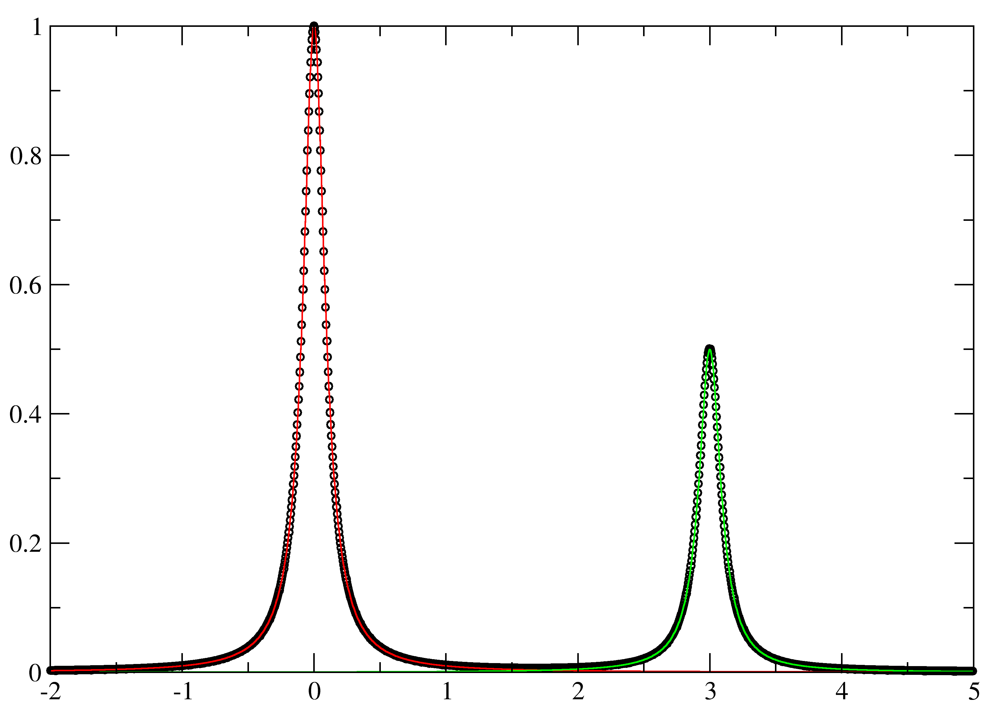
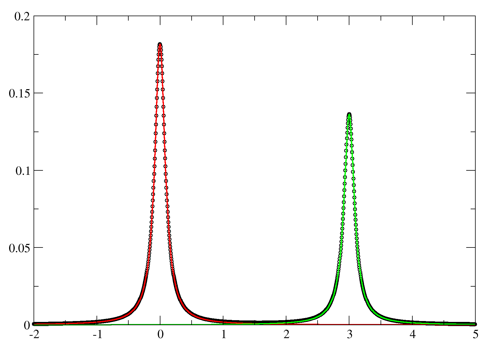
Here the uncommented line reads in the second spectrum from the block data for dat.txt, sim_a.txt and sim_b.txt. eg):

$ ./go_xmgr

Results in:

Additional Notes. We can easily expand the program to fit 3,4,5 etc resonances. There is also a version where one can fix the LW value to a defined value using the 3rd row in the "peaks.txt" file.

Appendix Files:

All of the files and source code for the tutorial are available here:

tut.zip

TABLE OF CONTENTS